AI Fundamentals

This page follows one LLM request from text on the screen to generated, streamed text.

The walkthrough uses a decoder-only, autoregressive text transformer with ordinary cached decoding. It is a common design, not a description of every language model or serving optimization.

Part 1 of 7: Fundamentals → Prompt engineering → Models and providers → Knowledge bases → Agents → Infrastructure → AWS AI Services.

Visual intuition: a journey through a learned world

Use the infographic below as an intuitive mental model for LLM inference. It gives you a way to picture how a trained model responds to a prompt and builds an answer one token at a time. The journey is only an analogy; the sections that follow explain the actual mechanics.

An intuitive mental model for how an LLM turns a prompt into a response

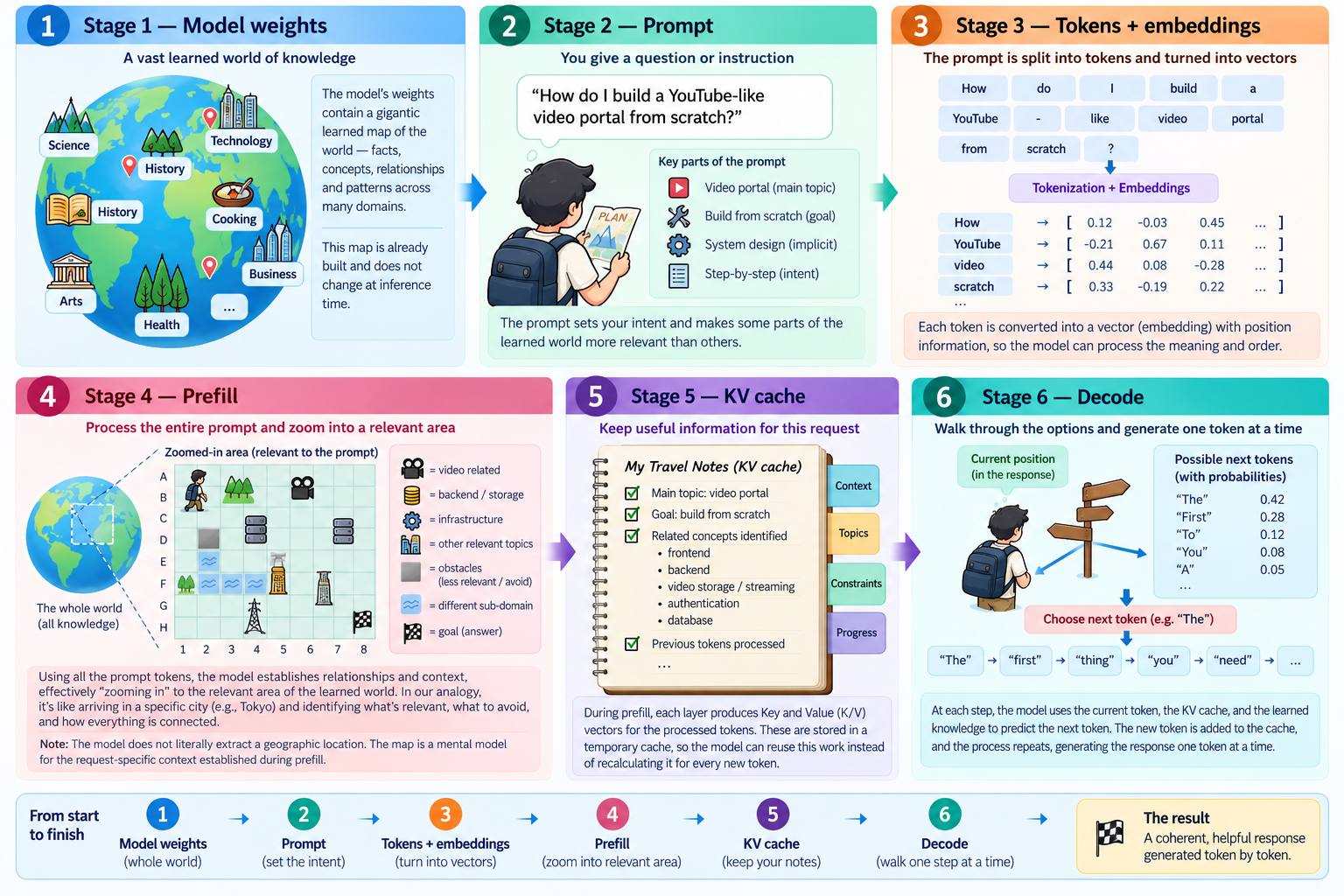
With that overall picture in mind, the rest of this page follows one simple prompt through every stage of the process:

"The capital of France is"

The model will complete this prompt one token at a time. Section 1 maps the complete request flow, and the remaining sections then walk through each stage in order.

1. Big picture: complete request flow

The prompt is processed once, then the generated token loops through the model until a stop condition is reached:

"The capital of France is"
        ↓ tokenizer
tokens → token IDs
        ↓ internal embedding lookup
vectors
        ↓ transformer / attention
contextual representation
        ↓ output projection
logits
        ↓ temperature → softmax
probabilities
        ↓ top-p / sampling
next token ID → " Paris"
        ↓ append to context and repeat
detokenize / stream text

• The values, IDs, and token boundaries on this page are illustrative; every model has its own compatible tokenizer and vocabulary.
• The surrounding application submits text and receives text. Its broader concerns—such as conversation history, permissions, tools, and validation—are supporting concepts later in the page, not steps performed inside this single inference loop.

🧠 Complete single-request sequence — the map for this page

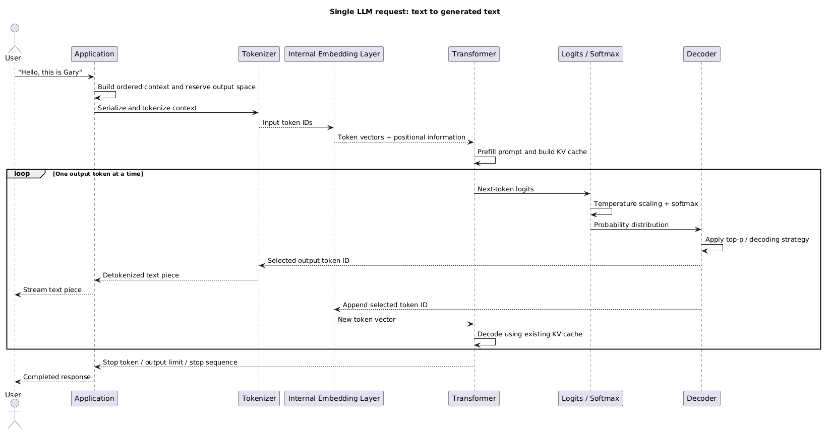
Before Stage 1 — construct the prompt

Before this text reaches the tokenizer, the application combines the user’s request with the task instructions, relevant context, optional examples, and desired output format. Learn how to design that input in AI Prompt Engineering.

2. Stage 1 — text becomes tokens and token IDs

• A tokenizer splits text using a vocabulary designed for that model.
• A token may be:
  • a whole word;
  • part of a word;
  • punctuation;
  • a whitespace pattern;
  • one or more bytes.
• Leading spaces can be part of a token, which is why examples often show tokens such as " Gary".

Illustrative tokenization:

"The capital of France is"
          ↓ tokenizer
["The", " capital", " of", " France", " is"]
          ↓ vocabulary lookup
[464, 3139, 286, 4881, 318]

• The numbers are illustrative; every tokenizer/model can assign different boundaries and IDs.
• A token ID is an integer index into the model vocabulary.
• 464 does not itself contain the meaning of “The”; it identifies the relevant vocabulary entry.
• Tokenization affects:
  • context usage and input cost;
  • truncation;
  • latency;
  • handling of code, URLs, identifiers, tables, and different languages.

3. Stage 2 — token IDs become internal vectors

• The transformer does not meaningfully reason over raw integers such as 464.
• The model contains a learned token-embedding table.
• The token ID selects one row from that table:

token ID 464
      ↓ embedding lookup
[0.83, 0.17, -0.31, ...]

• For our running request, each of [464, 3139, 286, 4881, 318] selects a learned vector.
• Each input token becomes a vector with the model’s internal hidden dimension.
• These vectors were learned with the rest of the model during training.
• The vectors begin as token representations; transformer layers then make them contextual.

Important boundary:

• Standard LLM inference normally uses the generation model’s internal embedding layer.
• It does not normally call a separate external embedding model before generation.
• A dedicated embedding model used for semantic search or a vector database is a different model and interface; see AI Knowledge Bases.

3.1 The model pipeline is coupled

• The tokenizer, vocabulary, internal embedding weights, transformer weights, output vocabulary, and detokenizer form one model-compatible pipeline.
• This coupling is model-specific or checkpoint/model-family-specific, not simply provider-specific.

                    MODEL / CHECKPOINT
                           │
          ┌────────────────┼────────────────┐
          ↓                ↓                ↓
 tokenizer/vocabulary  embedding table  transformer weights
          │                │                │
     token IDs       learned vectors   contextual processing
          └────────────────┼────────────────┘
                           ↓
                  vocabulary logits
                           ↓
                  matching detokenizer

• Token ID 464 only means something relative to its tokenizer vocabulary.
• Arbitrary token IDs from Model A cannot normally be supplied to Model B.
• The internal embedding table and transformer are trained together; GPT’s internal vectors cannot normally be substituted into Llama’s transformer, for example.
• Output logits correspond to the same model vocabulary, so generated IDs need the matching detokenizer.
• The concepts of softmax, greedy decoding, temperature, and top-p are general; providers decide which controls and implementations their serving APIs expose.
• Through an API, this coupled machinery is normally packaged behind a text/messages-in → text/tokens-out interface.

4. Stage 3 — prefill processes the prompt

Prefill is the initial forward pass over the supplied prompt, before the first response token is selected. Starting with the vectors from Stage 2, the model processes the prompt through its Transformer layers. This computes the context needed to predict the first new token and normally fills a key-value (KV) cache for later generation.

All five prompt tokens are already known, so their positions can be processed together within each layer. The layers still run in sequence. This differs from later decoding, where the next generated token must be selected before it can become the next input.

3 · Prompt pass›4 · Inside the Transformer→5 · Vocabulary logits

From Stage 2 · all five prompt vectors are ready

The●v₁

capital●v₂

of●v₃

France●v₄

is●v₅

↓↓↓↓↓

Prefill · run the prompt through the TransformerLayer 1 → Layer 2 → … → Layer N
Process the five positions together in each layer.
Stage 4 zooms inside this same pass.

↓ result for next-token prediction

★ Final hidden state at “is”
The last position can use “The capital of France is”.

↓

Stage 5: vocabulary scores
Stages 6–9 select the first new token:
" Paris"

↓ attention information saved along the way

KV cache for the prompt
Each layer saves its attention keys and values for the five positions.

↓

Reuse during decoding
Process the new " Paris" token using the saved prompt cache.
Continue this loop in Stage 10.

Prefill does the prompt's initial computation and saves attention work for reuse. Each dot represents a whole vector from Stage 2; text labels are for us, with leading spaces omitted.

Together does not mean looking ahead. A causal mask allows each position to use only itself and earlier positions: "The" can use only "The"; "is" can use all five prompt positions. No position can use " Paris" yet.

What is being “prefilled”? In typical cached generation, the attention cache is populated with the prompt’s computed keys and values. These are per-layer numerical features that later tokens can attend to, so the model can reuse earlier work. They are temporary computation for this context, not newly learned model weights. See how KV caching works.

Why the pause before the first token? The prompt pass must finish before the first response token can be selected. Longer prompts generally increase this work and cache memory. Time to first token (TTFT) includes prefill plus network overhead, tokenization, scheduling, and first-token selection.

Does every request process the entire prompt in one batch?

This example starts with no reusable cache. Serving systems may reuse a cached prefix or split a long prompt into chunks. Prefill still processes the supplied input that has not yet been cached, preparing it for subsequent generation.

5. Stage 4 — the transformer makes tokens contextual

What does the Transformer change? Each position’s initial representation becomes a context-dependent hidden state, also called a contextual representation. Follow the vector at "is": its token label stays the same, but the information represented by its numbers changes.

This is a closer look inside the prefill pass from Stage 3. The same Transformer layers also process each new token during the later decoding loop. Positional information supplies token order: some models add position vectors to embeddings; others apply position inside attention, such as rotary positions. “Embedding + position” below is a conceptual shorthand.

3 · Prompt pass›4 · Inside the Transformer→5 · Vocabulary logits

Before · Stage 2's vectors entering the prompt pass

Before at “is”: mainly its token embedding + position. It has not yet incorporated this prompt's preceding context.

The●v₁

capital●v₂

of●v₃

France●v₄

is●v₅

Self-attention at “is” combines information from relevant earlier positions and itself, using learned, context-dependent weights.

Transformer
Block 1

↓

Transformer
Block 2

⋮

Transformer
Block N

Each block updates all five representations. The paths above highlight only the information available at “is”.

↓

After · contextual hidden states

The●h₁

capital●h₂

of●h₃

France●h₄

is★h₅ = h

After at “is”: h encodes contextually useful information for predicting what follows “The capital of France is …”

Five vectors in → five contextual hidden states out, each still d_model dimensions. The star marks the final position we follow into Stage 5; it is still a vector, not a word.

The Transformer repeatedly transforms a sequence of vectors so that each position contains contextually useful information. Attention combines learned numerical features; it does not literally copy word meanings into "is". Each position can use only its own prefix, so "France" cannot use the later "is".

What happens inside each Transformer block?

Multiple self-attention heads combine information across allowed positions in different learned ways. Feed-forward layers then transform each position's features. Residual connections combine updates with earlier representations, and normalization helps keep activations stable. Repeating these operations across many blocks produces the final hidden states.

The dots and paths are an educational schematic, not literal vector geometry or measured attention strengths. Contextualization does not guarantee factual accuracy.

6. Stage 5 — output projection produces logits

How does a contextual vector become scores for words? Take h, the final hidden state at "is" from Stage 4. The output projection is a learned mapping from the hidden dimension to the vocabulary dimension: it produces one logit (raw score) for every vocabulary token, including word pieces and punctuation.

3 · Prompt pass›4 · Inside the Transformer→5 · Vocabulary logits

The●h₁

capital●h₂

of●h₃

France●h₄

is★h₅ = h

↓

Select the last position's final hidden state★ h = […, …, …, …]
d_model dimensions · after any final normalization

↓

Learned output projectionlogits = W_vocab · h + b
W_vocab: vocabulary_size × d_model · bias b is optional

↓

Vocabulary-sized vector of raw scores[…, -0.693, …, -1.386, …, -3.507, …]
vocabulary_size dimensions · one entry per token ID

Token / logit−4 0

" Paris"−0.693

" Lyon"−1.386

" Marseille"−1.897

" Berlin"−2.659

" Rome"−3.507

… every other vocabulary token also has a score.
Bars extend left from zero. Here, less negative = higher score; “ Paris” scores highest among the entries shown.

Illustrative values, reused in Stage 6. Five vocabulary entries are displayed, not the full vocabulary. Logits can be positive or negative; they are not probabilities and need not sum to 1.

This is not vector search. The model does not run “find the nearest word to h”. It multiplies h by a learned weight matrix to compute all vocabulary scores. Each row supplies a token’s scoring weights: a dot product with h, plus an optional bias. Although dot products also appear in similarity search—and some models share input embedding and output weights—this operation scores the fixed model vocabulary; it does not retrieve nearest words from a vector database.

★ Contextual hidden state h↓ Output projection → raw logits↓ Stage 6 · Temperature↓ Stage 7 · Softmax → probabilities↓ Stage 8 · Top-P → candidate tokens↓ Stage 9 · Sampling → " Paris"

The output projection has scored the next-token candidates; it has not selected one. The next four stages turn those scores into the sampled " Paris" in this walkthrough. For the underlying embedding, attention, and linear output mapping, see Attention Is All You Need, §§3.2–3.5.

7. Stage 6 — temperature

Temperature is applied at every generated-token step. It changes the shape of the logits before they become probabilities:

• Lower temperature concentrates probability on likely tokens; it does not make them factual.
• Temperature does not remove tokens or choose the next token by itself.
• T = 1 is the baseline: it leaves the logits unchanged. Values below 1 sharpen the distribution; values above 1, if an API allows them, flatten it. If your API only offers 0–1, then 1 is simply its least-conservative setting. This walkthrough compares 1.2, 0.9, 0.5, and 0.1.

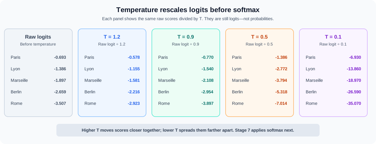
Continue the France request with these illustrative relative logits. For T > 0, temperature divides each logit by T: a lower T increases the separation between scores. If an API accepts T = 0, it usually selects greedy decoding rather than literally dividing by zero. Greedy decoding chooses a highest-scoring token; it is not an absolute reproducibility guarantee across serving implementations. Generation strategies.

Apply the setting to the task: standardized wording, such as a lease template, calls for low temperature (for example, 0.0–0.3 where supported); brainstorming may benefit from higher temperature (for example, 0.8–1.0). There is no universal 0.5 default that suits every task. Low temperature reduces variation but does not guarantee identical text, correct legal language, or an exact structure. Use approved templates and schema constraints where appropriate; maximum output tokens controls length. Bedrock inference parameters.

Token	Raw logit	÷ 1.2	÷ 0.9	÷ 0.5	÷ 0.1
" Paris"	-0.693	-0.578	-0.770	-1.386	-6.930
" Lyon"	-1.386	-1.155	-1.540	-2.772	-13.860
" Marseille"	-1.897	-1.581	-2.108	-3.794	-18.970
" Berlin"	-2.659	-2.216	-2.954	-5.318	-26.590
" Rome"	-3.507	-2.923	-3.897	-7.014	-35.070

These are still logits, not probabilities. The diagram shows only the Stage 6 rescaling; Stage 7 applies softmax next.

📐 Stage 6: temperature rescales logits only — no probabilities yet

8. Stage 7 — softmax produces probabilities

Softmax converts the adjusted scores from Stage 6 into probabilities. Written in terms of the raw logits zᵢ, the formula is pᵢ = exp(zᵢ / T) / Σⱼ exp(zⱼ / T). Temperature is applied once; the denominator includes every eligible vocabulary token.

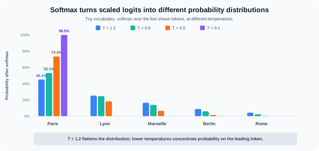
For the numerical examples in Stages 7–9, use a toy vocabulary containing only the five tokens below. Applying softmax to their rounded logits gives these approximate percentages. In a real full vocabulary, the other logits also contribute to the denominator; these five entries would not generally sum to 100%. Rounding can also make displayed totals differ slightly from 100%.

Token	temperature = 1.2	temperature = 0.9	temperature = 0.5	temperature = 0.1
" Paris"	45.1%	53.1%	73.4%	99.9%
" Lyon"	25.3%	24.6%	18.3%	0.1%
" Marseille"	16.5%	13.9%	6.6%	<0.1%
" Berlin"	8.8%	6.0%	1.4%	<0.1%
" Rome"	4.3%	2.3%	0.3%	<0.1%

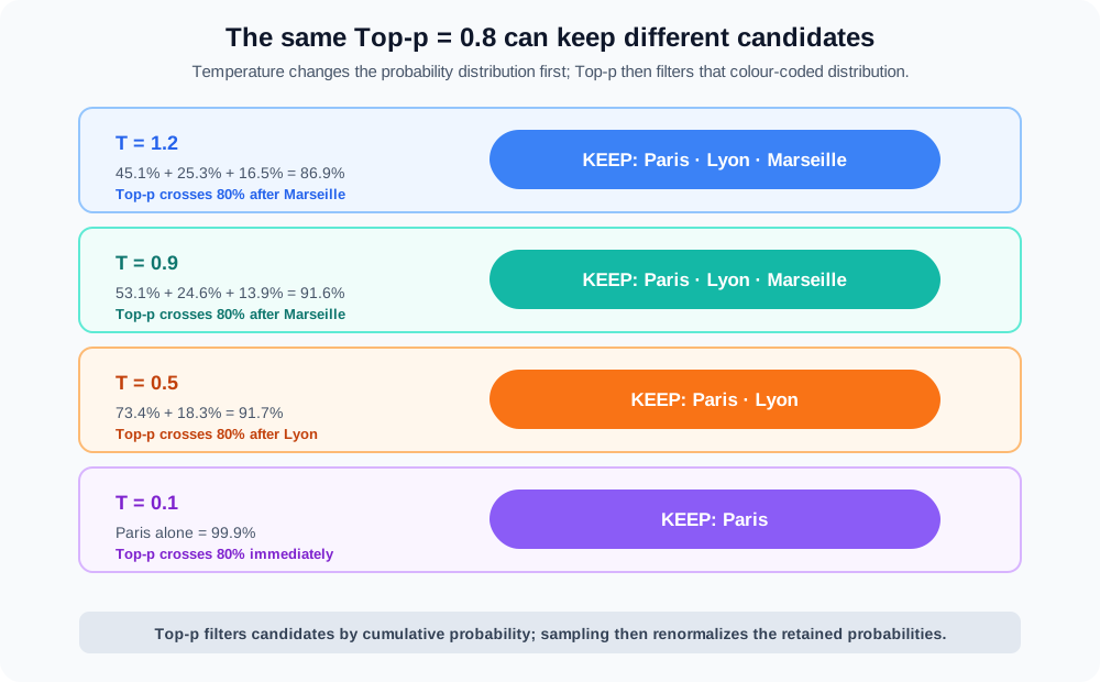
Only now do we have probabilities that top-p can use. To keep one concrete path through the later stages, use the orange temperature = 0.5 column below; the next diagram also shows how the top-p candidates change at 1.2, 0.9, and 0.1.

📊 Stage 7: softmax makes the temperature effect visible as probabilities

9. Stage 8 — top-p filters the sampling candidates

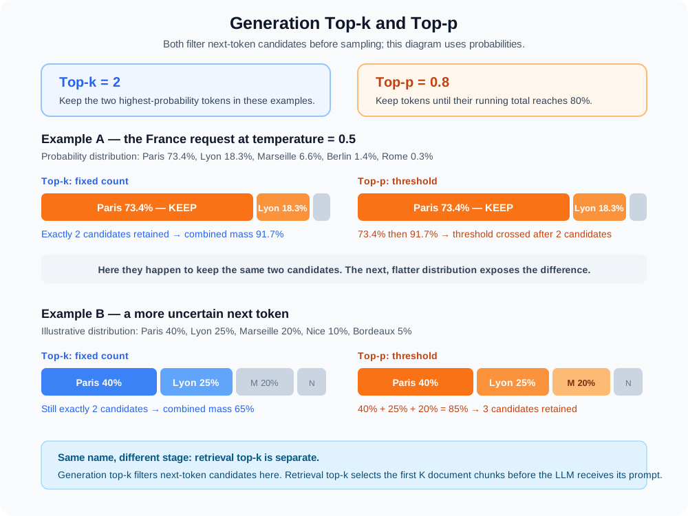
Apply top-p = 0.8 to the Stage 7 probabilities. Starting from the most likely token, keep tokens until their cumulative probability reaches at least 80%:

Tip: for a fixed probability distribution, higher top-p keeps at least as much probability mass and may keep more candidates. The retained set can stay the same until the threshold crosses another token.

How top-k and top-p differ — and can combine

Top-k restricts sampling to the k highest-ranked next-token candidates. This simple example has distinct scores and enough eligible tokens; tie handling and other filters can affect the final count in real implementations. Top-p keeps a variable number of candidates until their combined probability reaches p. When an API supports both, both can constrain the candidate pool; filtering order and renormalization are implementation-specific. Generation controls.

Setting	With the temperature = 0.5 probabilities below	What is fixed?
top-k = 2	keeps " Paris" and " Lyon"	The number of candidates: 2.
top-k = 3	keeps " Paris", " Lyon", and " Marseille"	The number of candidates: 3.
top-p = 0.8	keeps " Paris" and " Lyon" because their cumulative probability reaches 91.7%	The probability mass: at least 80%.
top-k = 2 and top-p = 0.8	both filters apply; the final pool cannot be wider than Top-k’s two candidates in this example	Both constraints.

Think of both together as a double boundary: Top-k prevents a pool from growing beyond a fixed count; Top-p prevents sampling from candidates outside its probability-mass cutoff. Top-k and top-p are decoding controls, not context length or retrieval top-k. Whether an API exposes either control, or allows both together, is model-specific.

🔢 Top-k sets the candidate count; ✂️ Top-p sets a probability-mass threshold; supported APIs can apply both

Cumulative probability is the running total in descending probability order: each row adds its probability to every row above it.

Token	Probability from Stage 7	Cumulative (running total)
" Paris"	73.4%	73.4%
" Lyon"	18.3%	91.7%
" Marseille"	6.6%	98.3%
" Berlin"	1.4%	99.7%
" Rome"	0.3%	100.0%

The threshold is crossed at " Lyon" (91.7%), so retain Paris and Lyon and exclude the remaining candidates. Top-p does not require any individual token to have an 80% probability.

✂️ With the same Top-p = 0.8, lower temperature reaches the threshold with fewer candidates

10. Stage 9 — sample the next token

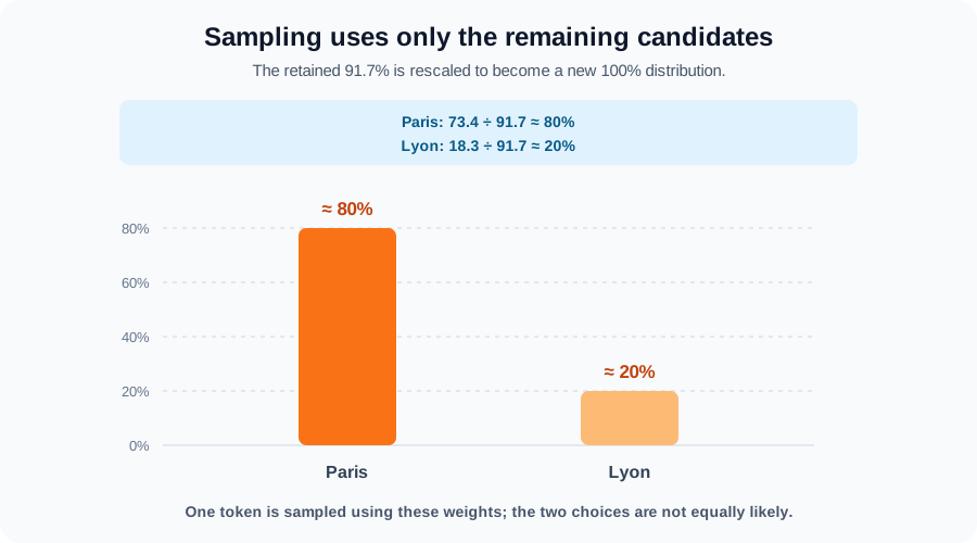
Continue the orange temperature = 0.5 path: only " Paris" and " Lyon" are eligible. Their probabilities are normalized within that candidate set—roughly 80% versus 20%—and one is sampled. They are not equally likely. In this walkthrough, sampling selects " Paris".

🎲 The retained probabilities are rescaled to 100%, then one token is sampled

The selected ID now becomes input to the next decode step.

11. Stage 10 — append the token and repeat autoregressively

The input/output distinction is fundamental:

• Input/prefill: many prompt tokens can be processed together.
• Output/decode: token N + 1 depends on token N, so generation is sequential.

"The capital of France is"
      ↓
predict token ID for " Paris"
      ↓ append to context
"The capital of France is Paris"
      ↓
predict token ID for "."
      ↓ append to context
predict end-of-sequence

• Every generated token becomes part of the context used to predict the next token.
• The KV cache lets decoding reuse attention information from previous tokens instead of recomputing the entire prefix each time.
• The new token must still pass through the transformer before the following token can be chosen.
• Time per output token (TPOT) measures the average decode time between generated tokens.
• TPOT is influenced by model size, serving hardware, batch/load, KV-cache size, and provider implementation.
• Because tokens are produced one at a time, the server can stream each completed text piece to the client instead of waiting for the full response.

The sequence is autoregressive, but some serving systems accelerate it using speculative decoding: a draft proposes several tokens and the target model verifies them together. Streaming chunks also need not correspond one-to-one with tokens. Assisted decoding.

12. Stage 11 — token IDs become text again and stream

• The decoder produces token IDs.
• The tokenizer maps each selected ID back to its token text/bytes and joins the pieces.

7123 → " Paris"
  13 → "."
        ↓ detokenize
"The capital of France is Paris."

• IDs are illustrative and model-specific.
• The output does not pass through an embedding model again.
• With streaming enabled, the application may receive and display decoded text pieces incrementally.
• A client may buffer incomplete byte/Unicode sequences so only valid text is displayed.

13. Supporting concepts beyond the single-request loop

The core journey ends when decoded text is streamed. The following material explains the surrounding constraints and related concepts without changing the inference path above.

13.1 Conversation, context, and context window

• Conversation: the logical history stored by the application or agent.
• Context: the tokens actually constructed and supplied to this particular model call.
• Context window: the model-defined maximum token budget available to one call, usually covering input context plus generated output.
• In the stateless request pattern illustrated here:
  • the model does not automatically retain the previous conversation;
  • the application stores messages or another memory representation;
  • the application selects and resends relevant history for the next call.
• Stateful APIs may let the client send a conversation/session identifier instead. The serving platform then manages history or cached state; this does not mean inference has trained that conversation into the model’s weights.

The application may build context from:

system/developer instructions
+ previous user messages
+ previous assistant messages
+ retrieved documents
+ tool definitions and tool results
+ current user message
+ space reserved for generated output

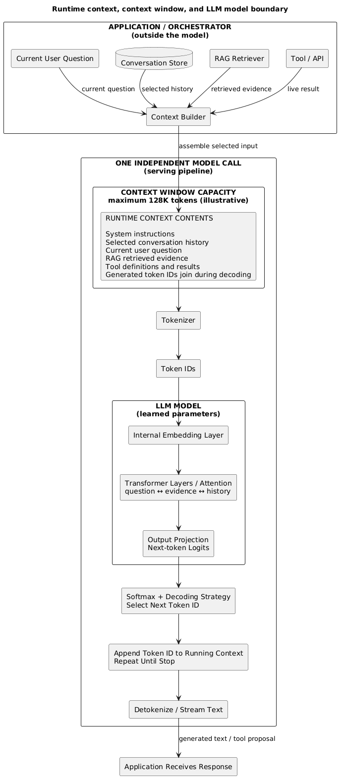
• Runtime context is the actual content assembled for one LLM invocation; generated token IDs join the running context during decoding.
• Runtime context = contents. Context window = maximum capacity.
• A 128K context window in the diagram is illustrative; limits differ by model and may include separate output constraints.
• RAG and tools run outside the model, then add retrieved evidence or tool results to that context.
• The transformer has no special “RAG mode”: after tokenization, attention processes evidence, history, instructions, and the question as tokens in the same context.
• Model parameter count and context-window size are separate:
  • parameters are learned weights inside the model;
  • the context window is the per-request token budget.

🧩 Runtime context: application inputs become one LLM request

• Python analogy:

MAX_CONTEXT_TOKENS = 128_000  # illustrative model limit
model_parameters = load_learned_weights()

def llm_call(input_tokens, max_output_tokens):
    assert len(input_tokens) + max_output_tokens <= MAX_CONTEXT_TOKENS
    running_context = list(input_tokens)

    for _ in range(max_output_tokens):
        logits = model_forward(model_parameters, running_context)
        next_token_id = decode(logits)
        if is_stop_token(next_token_id):
            break
        running_context.append(next_token_id)
        yield detokenize(next_token_id)

• model_parameters stay fixed during inference; running_context is different for every call and grows during generation.
• The pseudocode shows the mental model; production serving normally reuses a KV cache rather than recomputing the entire prefix.

• A real streaming detokenizer may buffer multiple tokens/bytes before emitting valid text; stop sequences may also span several tokens.

• The selected context is serialized according to the model’s chat format, tokenized, and supplied to a new inference call.
• Message roles are structured context conventions:
  • system/developer: application behaviour and constraints;
  • user: caller request and data;
  • assistant: earlier or generated model output;
  • tool: observation returned by external execution.

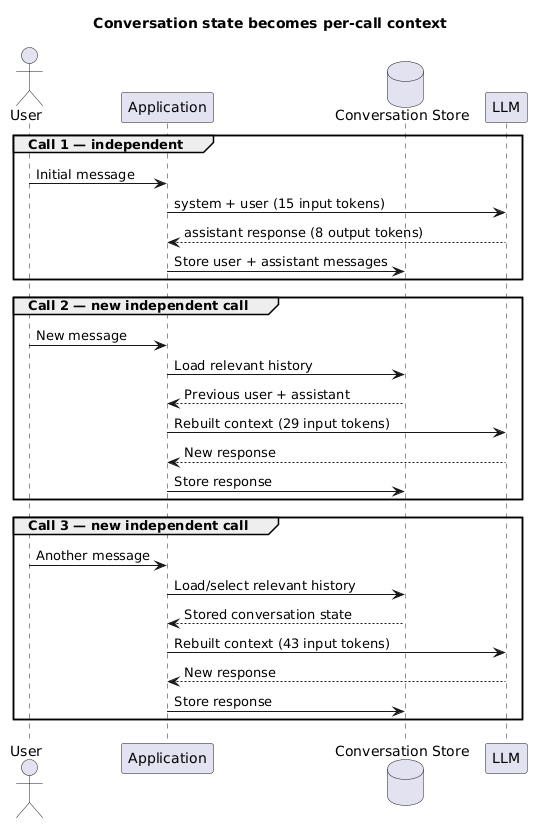
13.2 A 1,000-token calculation

The diagram used 128K to show the boundary. Shrink it to 1,000 tokens to make the same capacity calculation easier to follow:

input context tokens + generated output tokens ≤ context window

In this stateless example, the application builds each request independently; resending selected history usually makes later input contexts larger:

CALL 1 — independent request
Input context: [system + user] = 15 tokens
Output:                              8 tokens
Total used:                   15 + 8 = 23 / 1,000
Unused capacity:            1,000 - 23 = 977 tokens
Application stores the 8-token assistant response.

CALL 2 — new independent request
Input context:
[system + previous user + previous assistant + new user] = 29 tokens
Theoretical output headroom:                    1,000 - 29 = 971 tokens
Application stores the new response.

CALL 3 — new independent request
Input context:
[previous context + previous response + new message] = 43 tokens
Theoretical output headroom:                    1,000 - 43 = 957 tokens

• The previous output consumed Call 1’s budget while it was generated.
• If the application resends that output in Call 2, it is counted again as part of Call 2’s input context.
• Theoretical headroom is not necessarily the allowed output size:

available output budget = minimum of:
  configured max output tokens
  model/provider output limit
  context window - input context tokens

💬 Conversation history and independent context windows

• Practical consequences:
  • longer context increases input tokens, cost, prefill work, TTFT, and KV-cache memory;
  • output capacity must be reserved;
  • excess history must be trimmed, summarized/compacted, or retrieved selectively;
  • important evidence can be buried in irrelevant or repeated content;
  • a larger advertised window does not guarantee reliable attention to every detail.
• A provider may manage conversation history or cached session state between API calls. That state belongs to the application/serving platform; ordinary inference does not train it into model weights.

14. Training, fine-tuning, and inference

• Pretraining learns model parameters from broad data.
• Fine-tuning updates parameters for a more specific behaviour or task.
• Inference uses those parameters to generate output; the request changes context, not weights.

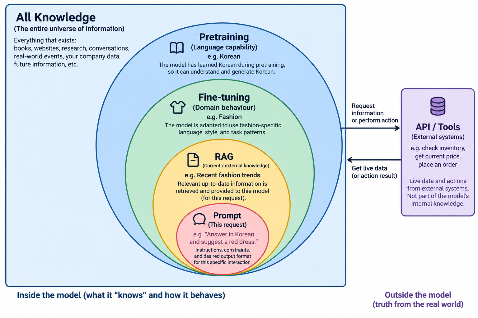
The Korean-fashion example shows how a trained model can be combined with retrieved evidence, a prompt, and external tools. The choice of adaptation method belongs in Models: prompt engineering, RAG, or customization.

The nesting below shows conceptual scope, not literal data containment: each inner layer narrows what is used for the current task.

🧩 Model + context narrows toward this request; API / Tools remain outside the model

14.1 Apply it: a Korean fashion assistant

For “한국어로 최근 트렌드를 요약하고 빨간 옷을 추천해 주세요,” the application can retrieve trend documents with RAG, look up a live price and stock through an API, then instruct the model to answer in Korean. These techniques complement one another; they are not alternatives.

14.2 How models learn

Training describes when weights change; the learning method describes where the teaching signal comes from.

Method	Teaching signal	Example
Supervised learning	Examples paired with target labels or values	Emails labelled spam/not spam; house attributes paired with sale prices. Classification predicts a category; regression predicts a number.
Unsupervised learning	Unlabelled data, with an objective that discovers structure	Cluster customers by purchasing patterns without supplying customer-segment labels.
Self-supervised learning	Targets constructed from the data itself	Hide a word and predict it, or use earlier tokens to predict the next token. Human annotators do not label every training example.
Reinforcement learning (RL)	Rewards from actions and outcomes	Learn a policy that chooses actions to maximize expected cumulative reward. A reward can be delayed; it need not specify the correct action at every step.

LLM next-token pretraining is self-supervised: text supplies both the input and target. Instruction examples can then support supervised fine-tuning, followed by preference-based post-training. Self-supervision is often grouped with learning from unlabelled data, but its explicit prediction targets distinguish it from ordinary clustering. Sources: Google’s learning-method overview and self-supervised learning glossary.

14.3 Bias, variance, and generalization

Concept	Meaning	Typical symptom	Possible response
High bias	Restrictive assumptions miss the underlying relationship	Underfitting: poor training and validation results	Improve features, increase suitable model capacity, or reduce excessive regularization.
High variance	Learned predictions change too much with the training sample	Overfitting: strong training results but weak validation results	Add representative data, regularize, simplify the model, or use suitable ensembles.

For squared-error prediction, the classical decomposition is expected error = bias² + variance + irreducible noise. Reducing one component can increase another; compare held-out performance rather than maximizing training accuracy. A training/validation gap is a diagnostic clue, not proof: leakage, distribution shift, and label errors also need investigation. scikit-learn’s bias–variance example.

Statistical bias is different from unfair demographic bias. A model can generalize well overall and still perform poorly for a particular group. Measure group outcomes under responsible AI.

14.4 Related ML vocabulary

Concept	Recognition rule
Overfitting	Very high training performance but weak performance on unseen validation/test data; excessive complexity for the amount of training data increases the risk.
Underfitting	Poor performance on both training and unseen data; often too simple or insufficiently trained.
GAN	A generative-model training approach; see generative model families for the generator/discriminator relationship.
Regularization	Constrains learning to reduce overfitting; it is different from the reward signal that defines desired RL outcomes.

Continue to training/validation/test sets, regularization versus reward, and reinforcement learning from human feedback to connect these concepts to model adaptation.

For deeper treatment, see AI Knowledge Bases, AI Agents, and AI Infrastructure and Evaluation.

15. Hallucination, grounding, and structured output

• The model selects plausible next tokens from learned patterns and supplied context; it does not automatically verify claims.
• A hallucination can be fabricated or factually incorrect content, or output that contradicts or goes beyond the source material it was required to use. Definitions vary by task, so distinguish factual correctness from faithfulness/grounding in supplied evidence. Hallucination taxonomy.

Fictional example:

Question: "Who is the CEO of Glucolte?"
Trusted evidence in this request: none

After "The CEO of Glucolte is ..."
illustrative next-token probabilities:
  "Gary"     38%
  "John"     21%
  "Michael"  12%
  ...

Generated answer: "The CEO of Glucolte is Gary Lu."

• The probabilities are illustrative; names may also span several tokens.
• The answer is grammatical and may sound confident, but this example supplies no evidence establishing the person’s role. It is ungrounded in the request; that alone does not establish that it is false. A model can answer some questions correctly from learned knowledge without retrieved context. An evidence-only task must still reject unsupported assertions.

• The model does not reliably apply fact unknown → stop; the same next-token process from the walkthrough still applies.

• Unsupported output can arise because:
  • the fact was absent, incorrect, or stale in training data;
  • the request context is missing or conflicting;
  • retrieval returned irrelevant or outdated evidence;
  • the model ignored or incorrectly combined valid evidence.
• RAG can reduce hallucination risk by supplying evidence, but retrieval can fail and the model can misuse correct evidence. RAG evaluation measures these separately.
• Low temperature does not solve this:
  • it makes high-probability continuations more likely;
  • a likely continuation can still be wrong;
  • the model may repeat the same wrong answer more consistently.
• Reduce risk by:
  • supplying authoritative evidence through retrieval or tools;
  • requiring an insufficient-evidence response;
  • carrying source IDs into citations;
  • validating calculations, identifiers, and business rules in code;
  • using human approval for high-impact outcomes.
• Structured output constrains syntax or shape, not truth:
  • valid JSON can contain a nonexistent customer;
  • schema-valid tool arguments can still be unauthorized or unsafe.

16. What remains outside the model

The model proposes output. The application decides which evidence to supply, which actions to execute, and whether the result is acceptable. Continue with the page that owns each responsibility:

• Retrieval internals: AI Knowledge Bases
• Tool loops and agents: AI Agents
• Production controls: AI Infrastructure and Evaluation